在分析数据集时,常常会碰到一些缺失值,如果缺失值的数量相对总体来说非常小,那么直接删除缺失值就是一种可行的方法。但某些情况下,直接删除缺失值可能会损失一些有用信息,此时就需要寻找方法来补全缺失值。
安装包 1 2 conda create -n mice conda-forge::r-tidyverse conda-forge::r-irkernel conda-forge::r-mice conda-forge::r-vim"IRkernel::installspec(name='mice', displayname='mice')"
导入数据 1 2 3 4 5 6 7 8 9 10 library( tidyverse) %>% head( ) ( airquality) <- str_replace_all( colnames( airquality) , pattern = '\\(| |-' , replacement = '_' ) ( airquality) <- str_replace_all( colnames( airquality) , pattern = '\\)' , replacement = '' ) %>% summarise_all( ~ round ( sum ( is.na ( .) ) / length ( .) , 3 ) ) <- airquality %>% ( Month = factor( Month) ) %>% ( Day = factor( Day) )
查看数据质量 1 mice:: md.pattern( airquality)
左边第一列,为样本数 右边第一列,为累积缺失值个数,0为没有缺失。 第一行可以理解为,有111条记录,所有列都有值,没有缺失值。 第二行可以理解为,有35条记录,Ozone列有缺失值。 1 2 options( repr.plot.width = 12 , repr.plot.height = 12 ) :: marginmatrix( airquality)
当同一侧红蓝箱线图较为接近时可认为其对应考察的另一侧变量缺失情况比较贴近完全随机缺失,这种情况下可以放心大胆地进行之后的插补,否则就不能冒然进行插补。
1 2 options( repr.plot.width = 6 , repr.plot.height = 6 ) :: fluxplot( airquality)
通量图可用于发现潜在的预测因子、更容易被预测的变量以及干扰插补模型的变量。一般来说,离对角线较近的变量通常比距离较远的变量关联性更好(关联性好的预测性更好),位于较低区域(尤其是左下角附近)且对后续分析不感兴趣的变量最好在插补之前从数据中删除。
mice包介绍 mice包实现了,多变量缺失数据填补的方法,基于多元回归模型来预测,每个不完整变量由单独的模型估算,进行多重混合评估。mice包算法可以实现对于连续型,二进制,无序分类和有序分类数据的进行混合。此外,mice包可以处理连续的两级数据,并通过被动插补来保持插补之间的一致性,通过各种统计诊断图,保证插补数据的质量,该包论文在统计软件领域顶刊JSS上。(from 粉丝日志 )
对于缺失值数据的处理,用3个步骤来进行定义。
填充:mice()函数,从一个包含缺失数据的数据框开始,然后返回一个包含多个完整数据集的对象,每个完整数据集都是通过对原始数据框中的缺失数据进行插而生成的。 分析:with()函数,可依次对每个完整数据集应用统计模型,分析填充的结果。 优化:pool()函数,将这些单独的分析结果整合为一组结果,最终模型的标准误和p值,都将准确地反映出由于缺失值和多重插补而产生的不确定性。 1 van Buuren, S., & Groothuis-Oudshoorn, K. (2011). mice: Multivariate Imputation by Chained Equations in R. Journal of Statistical Software, 45(3), 1–67. https://doi.org/10.18637/jss.v045.i03
进行迭代插补 1 2 3 4 5 6 7 8 9 10 11 <- c ( 'Month' , 'Day' ) <- mice:: quickpred( airquality, mincor = 0.1 , minpuc = 0 , include= "" , exclude = irrelevant_variable, method = "spearman" ) %>% as.data.frame %>% sapply( sum ) %>% t %>% as.data.frame %>% sapply( sum )
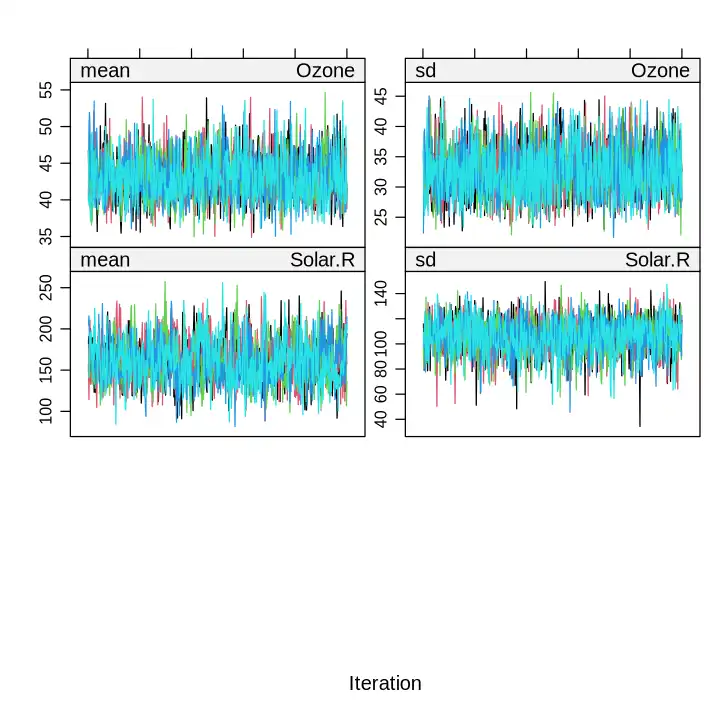
1 2 3 4 5 6 7 8 9 10 11 12 13 14 15 16 17 18 19 20 21 22 <- mice:: mice( airquality, predictorMatrix = predictorMatrix, maxit= 0 , seed= 1337 ) $ loggedEvents $ method[ c ( 'Ozone' , 'Solar.R' ) ] = 'cart' <- mice( airquality, method = init$ method, predictorMatrix = init$ predictorMatrix, m= 5 , seed= 1337 , maxit= 500 ) ( repr.plot.width = 6 , repr.plot.height = 6 ) ( imputed)
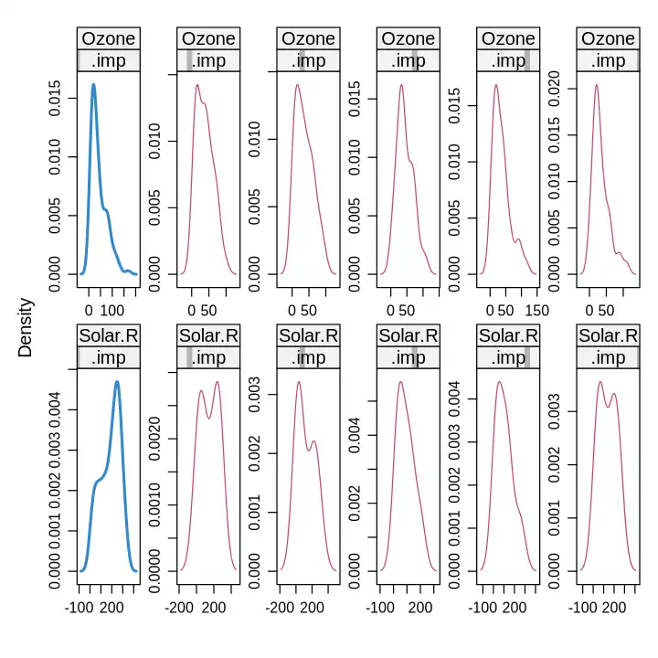
选择合适的插补(看图) 1 2 mice:: densityplot( imputed, ~ Ozone + Solar.R | .imp)
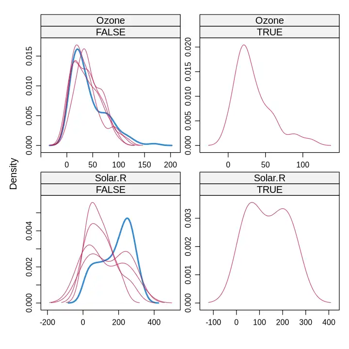
1 2 mice:: densityplot( imputed, ~ Ozone + Solar.R | .imp == 5 )
导出插补后的数据 1 2 3 4 5 6 7 8 9 f_mice_complete <- function ( l_data, l_imputed, l_colname, action) { [ rownames( l_imputed$ imp[[ l_colname] ] ) , l_colname] <- l_imputed$ imp[[ l_colname] ] [ action] return ( l_data) } <- imputed$ data<- f_mice_complete( Data, imputed, 'Ozone' , 4 ) <- f_mice_complete( Data, imputed, 'Solar.R' , 2 )
插补的不确定性 1 2 3 4 5 6 fit1 <- with( imputed, stats:: lm( formula( 'Ozone ~ Solar.R + Wind + Temp' ) ) ) <- with( imputed, stats:: lm( formula( 'Solar.R ~ Ozone + Wind + Temp' ) ) ) :: pool.r.squared( fit1) :: pool.r.squared( fit2)
插补数据集分析 1 2 3 4 5 6 7 8 9 10 11 12 13 14 15 16 17 fit <- with( imputed, ...) <- pool( fit)
插补的环境 1 2 3 4 date( ) for ( packagename in ( .packages( ) ) ) { ( packageDescription( packagename) ) }